Quality Control
1. PST STATION QUALITY CONTROL
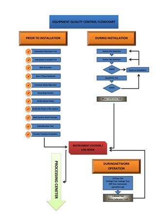
Before giving the green light for PST station to start providing data we are making a lot of tests. These tests are depicted in the following FLOW CHART.
2. SEISMIC RECORDER QUALITY TEST
a) Instrument Impulse Test
Setting the signal generator producing a square waveform with a frequency 0.1Hz, is like producing pulse signals every 10 sec. The three rescoring channels of the seismograph (sensor + digitizer/recorder) will be driven from this signal and the output will be monitored in DataMonitor. The data will be also recorded into micrSD flash card for further processing.
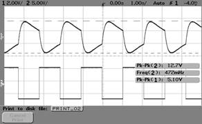
Input signal and system impulse response
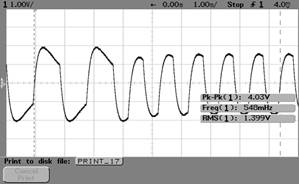
Impulse response low to med frequency
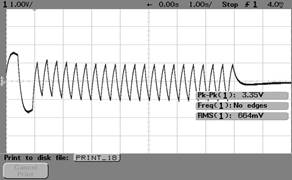
Impulse response med to high frequency
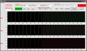
Impulse response plotted on DataMonitor
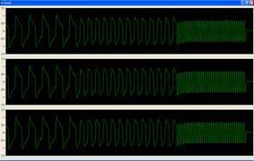
Impulse response plotted on data file
b) Instrument Distortion Test
For this test we inject sinusoidal signal at all recording channels of the instrument. The signal is recorded into recorder’s microSD flash card and then further processing can be done using Matlab.
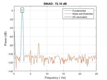
Instrument Distortion
c) Instrument Crosstalk Test
We can apply this test only between ant single instrument channels. Crosstalk between instruments os zero because they are located in different places.
To estimate crosstalk, a single sinusoidal signal from a signal generator is necessary to be injected at each recording channel. A fast crosstalk test can be done using DataMonitor2 software which plots in real time signal spectrum on screen so crosstalk level will be directly estimated.
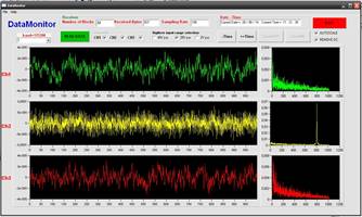
Instrument crosstalk on DataMonotor
Reading the data from the microSD flash the user can apply in depth signal processing and calculate crosstalk level
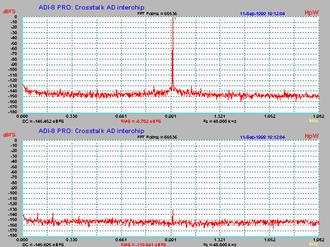
Instrument crosstalk
d) Instrument RMS & Offset Test
Instrument offset voltage and RMS noise can directly be derived from the recording signal, when no sensor is connected at the input. A fast offset calculation can be done using DataMonitor operating with “DC removal” unchecked, allowing the DC level to be plotted on the screen.
Fast RMS noise can also be performed using DataMonitor software operating with “DC removal” unchecked, in order to be able to apply auto-zoom in the recording signal and plot the peak-to-peak noise. Further processing can be done at the recorded data using matlab for extracting accurate DC level and RMS noise level.
e) Gain Accuracy & Gain/phase similarity
For this test we inject sinusoidal signal at all recording channels of the instrument. DataMonitor software gives us a quick result of the gain accuracy of the three recording channels. Repeating the test to all the instruments we can have a total gain accuracy of all the microseismic network. Further alanysis of the gain can be done by analyzing the recording signal with Matlab.
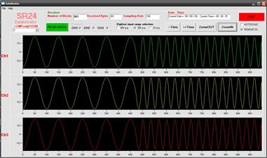
Gain/phase similarity on DataMonitor
g) Common mode rejection
This test can be applied only for the differential digitizer. Not possible to be applied when the sensor force-balance front end is present because it provides a single – ended input. To perform this test, equal signal must be injected at both digitizer’s differential input. The recording result presents the common mode rejection ratio of the digitizer.
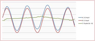
Common mode rejection
h) Recording polarity
The recording polarity is verified during the weight drop test. The weights first drops among the north side of the sensor and then drops among the east side of the sensor.
The weight should drops at double distance from the sensor installation depth. So if the sensor is installed at 10m, the weight should drop at 20 meters from the surface of the borehole.
We determine the direction of the first wave recorded by the weight drop. A north side drop will produce a wave with opposite direction of the Y axis (N-S axis). So it will produce a record which the first arrival will be downwards at NS channel.
Similarly, an east side drop will produce a wave with opposite direction of the X axis (E-W axis). So it will produce a record which the first arrival will be downwards at EW channel.
To verify vertical polarity, the weight must drop just next to the borehole at the surface. It will produce a record which the first arrival will be downwards atVertical channel because the produced wave will travel; downwards, so opposite of the direction of the Z axis.
i) Verify system delay
The system is synchronized with GPS time. Any possible delay might be because of the DPLL drift. It is described at “Main system clock precision” paragraph.
k) Verify the phase of the system.
This is a very difficult test that requires seismic shaking table, and one auxiliary recorder with three single ended inputs. Both recorders must be GPS synchronized. This test It can be performed only in our factory. We use the auxiliary recorder for direct sensor signal recording while the under test recorder, operates as a seismograph (sensor + digitizer/recorder). The shaking table shakes the sensor. Sweep frequency is 20sec to 200Hz. Once sweep is finished, we use matlab to process the data of the auxiliary and under test recorder. The phase has the shape of the following picture.
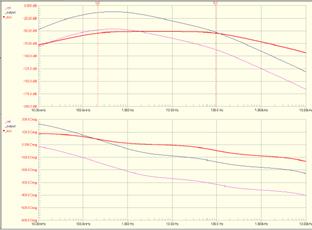
System Phase
l) Main system clock precision
The digitizer gives the ability for self drift calculation. Looking at the instrument’s log file, the overall drift between GPS cycles is always monitored. It is recorder in HEX format. For calculation the drift in microseconds, the user first has to convert the hexadecimal number into decimal, and then fivide by 115.200. For example if the hourly drift is hex0012, the drift is:
H0012 = DEC18
18/115.200 = 1.041usec
3. PST RESULTS QUALITY CONTROL
Before delivering a 3D final model to our clients we perform certain quality control tests which assure the 100% reliability of our results. These tests are:
- Resolution tests
- Checkerboard synthetic tests
- Ray coverage per cell tests
- Impulse response tests
- Ray tracing tests
- DWS and RDE tests
- Input data tests
RESOLUTION TESTS
The influence of systematic and random errors on the final Passive Seismic Tomography (PST) results is hard to quantify owing to the nonlinear nature of seismic tomography, the difficulty of quantifying noise in the input data, and the effect of parameterization. LandTech has designed an integrated resolution test procedure which quantifies the accuracy of PST results prior to submitting the final models to its clients.
A number of empirical methods of uncertainty estimation are used to ensure that only robust, well-constrained features of the final model are interpreted. They are based on the definition of artificial models with known distribution, dimension, and intensity of anomalies.
The procedure presents two steps: Initially, we solve the direct problem to determine synthetic travel times and then utilize those data as input for the inverse problem. The source–receiver geometry and inversion parameters are as close as possible to those used for the real data. The comparison of the final model with the initial (known) model provides a qualitative indication about the resolving capabilities.
Comparison between real model and that derived from the inversion of synthetic travel times.
Regions where the recovered model closely matches the input model are considered as well resolved. However, the degree of recovery is sensitive to the geometry and magnitude of the synthetic anomalies. These factors also have to be considered when interpreting the tests.
CHECKERBOARD TESTS
We build a checkerboard model characterized by alternated positive and negative anomalies of ±10% with respect to the initial 1D velocity model previously obtained. In this model, with the same configuration of earthquakes and stations as in the real inversion (we use the same hypocenters of the recorded earthquakes and station locations), we generate synthetic seismograms. In each one of the synthetic seismograms we measure the P- and S-wave arrival times and we use them to perform a synthetic passive seismic tomography inversion. We, then compare the obtained 3D tomographic model with the initial (checkerboard one) at various depths.
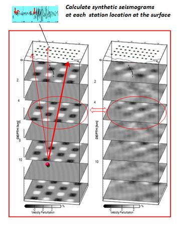
Example of a checkerboard test. We start from the recorded hypocenters embedded in a “checker board velocity model”; We calculate synthetic seismograms at each one of the installed stations; We determine P- & S-wave arrivals and invert for the velocities; Finally we compare the calculated structure with the original.
The illustrations right below present, results of the checkerboard test for a layer at 1.5 km and 3.5 km depth, respectively. In this example we can verify that all embedded artificial features (anomalies) in the velocity model are sufficiently recovered.
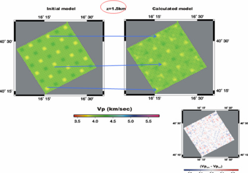
(a)
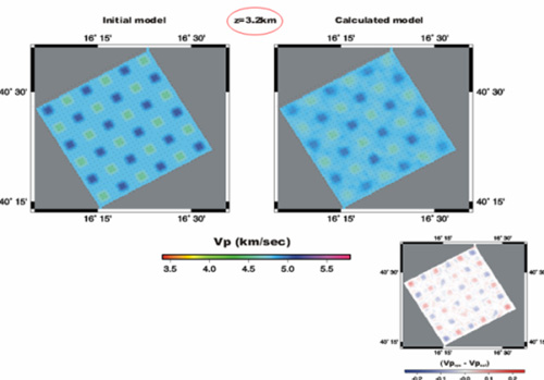
(b)
Results of checkerboard tests at a depth of a)1.5 km and b) 3.5 km. Also the % difference between the real and calculated velocities is depicted.
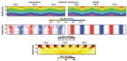
IMPULSE RESPONSE TEST
An important factor that determines the quality of the final tomographic model and the obtained resolution is the number of ray parameters that pass throughout each tomographic cell that is used for the inversion. By calculating the density of ray coverage all over the inverted block we have an additional measure to assess the reliability of our results.
RAY DISTRIBUTION TESTS
For the impulse response tests, we generate smoothed spot like anomalies at different locations in the domain. These anomalies have to be reproduced in the final models. The resolved volume has to coincide with the high coverage area, as in the checkerboard tests.
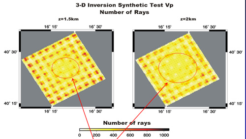
Red arrows show low ray coverage regions.
As an additional test, we calculate travel times in a velocity model equivalent to the obtained from the PST model. With this analysis we are able to check how well the inversion performs using anomalies with dimensions and positions similar to what we expect to deal with in the real medium. The parameter selection and inversion scheme were the same as in our 3D inversion.
We add noise to the synthetic travel times in order to simulate the uncertainties in the real arrival time data. The noise level is inversely proportional to the quality assigned to the arrival time picks. To obtain a statistically robust estimate, this procedure is repeated to generate an adequate number of noisy travel time datasets. When inverted, they generate a set of output models that mast show very slight differences among them.
To compare the models, we use slowness rather than velocity because it shows a clearer Gaussian distribution of the final results. The standard deviations of slowness for each node must be adequately small.
RAY TRACING TESTS
Here we investigate the effect that various ray tracing methodologies used during the inversion process can affect the accuracy of the derived models.
In the following example we compare some results from a real case study were we used 2 common ray tracing algorithms.
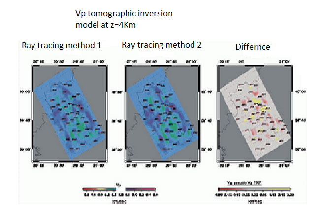
Comparison of inversion results using 2 ray tracing algorithms.
Comparing the obtained results we can see that they are similar as far as the cross section image is concerned, they differ slightly in the minimum and maximum velocity values. More precisely from the difference diagram between the Vp velocities estimated by the two methods we conclude that the minimum and the maximum velocities present smaller variations in the case of the second method.
DWS - RDE TESTS
Furthermore as an additional check for control we calculate a) the spread function b) the diagonal elements from the matrix RDE (Resolution Diagonal Elements) and c) the weighted sum of the seismic rays per unit mesh DWS (Derivative Weighted Sum). The values RDE, DWS and Spread depend on different factors such as the cell sizes of the mesh and the ray tracing scheme used. Figure 5.6.1 demonstrates an example representing the distribution of the above functions for the a Vp velocity model at depths 4km. Diagrams all over the depths of interest are calculated.
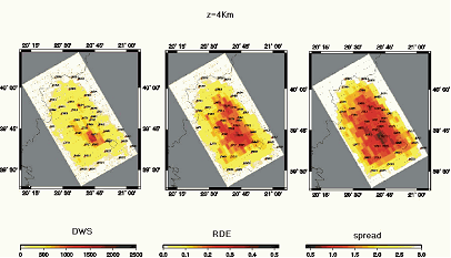
Plots of DWS, RDE and spread, for Vp model at 4km depth.
INPUT DATA TESTS
Here we assess the effects of the starting model and database characteristics. First, we perform the inversion using different trial structures as initial models. We perturbed the minimum 1D model by ±10% , and calculate the corresponding P-wave velocity structures. The results of this test indicate if the positions and shapes of the anomalies do not significantly change inside the studied volume.
Next, we analyze the control exerted on results by the database selection. We use a variation of the classical jack-knife test. A strong advantage of this method is that it does not require an estimate of noise in the data to assess the uncertainty in the resulting model because the noise itself contributes to the variance in the derived models. We perform an adequate number of inversions, removing a random10% of the initial dataset, and then examining the variance of the derived models.
The standard deviations among these models could be assumed as a measure of the uncertainty in the final model. Standard deviations for slowness among the final models are calculated at each node.